When I entered graduate school, I knew next to nothing about functional magnetic resonance imaging (fMRI) and it's history. I eventually began to piece together a picture of fMRI's more recent history as I started to notice certain topics permeating conferences, classes, and conversations. Even so, I've long been curious about what topics shaped the fMRI and MRI literatures over time. When I learned about burst detection, I immediately wanted to use the method to create a data-driven timeline of fMRI.
(You can view the Jupyter notebook I made to run all the analyses here. If you want to read more about burst detection, you can read this blog post, and if you want to apply burst detection analysis to your own data, you can download the burst detection package I compiled on PyPi.)
DATASET oF MRI ARTICLES
I used the PubMed database to collect the titles of MRI articles. I searched for the terms "fMRI" or "MRI" in the title/abstract field and restricted the results to articles and review papers published between 01/01/1987 and 11/30/17 and written in English. PubMed expanded the search to documents including the phrases "magnetic resonance imaging" or "functional magnetic resonance imaging" in the title or abstract. The search returned a total of 410,100 documents (accessed on 12/15/2017).
I only kept articles with publication dates that included a month and a year. Articles that had no publication date at all, no publication month, a season rather than a month, or that were published outside the date range were discarded, leaving a total of 371,244 documents.
If we look at how many MRI articles were published every month during the timeframe, we can see an almost linear (maybe exponential) increase in the number of articles published from 1987 to 2015, and then a slight decline. I don't know if this decline is due to some shift in the field -- maybe fewer articles contain the terms "fMRI" or "MRI" now or maybe fewer fMRI articles are being published -- or if it's reflective of some sort of delay in PubMed's indexing of articles.
It looks like approximately (a whopping!) 2000 MRI and fMRI articles have been published every month since 2014. That is much more than I would have guessed. Granted, these may not all be actual MRI or fMRI studies. The search returned all documents that contained fMRI or MRI in the title or abstract, but it's unclear whether those articles published new results or simply referenced previous studies.
PREPROCESSING ARTICLE TITLES
Since this analysis tracks how often different words appear in MRI article titles over time, I first had to preprocess the titles in the dataset. Preprocessing was pretty minimal -- I simply converted all words to lowercase, stripped all punctuation, and split each title into individual words. The titles in the dataset contained 101,843 unique words. A large chunk of these words only appeared a few times. Since I'm interested in general trends, I don't really care about words that rarely appear in the literature. In order to weed out uncommon words and reduce computation time later on, I discarded all words that appeared fewer than 50 times in the dataset. That left 6,310 unique words.
I was curious about what words are used the most in MRI and fMRI article titles. Not surprisingly, some of the most common words were magnetic, resonance, and imaging (which were part of the search terms) and common articles and prepositions, such as the, of, and a. Ignoring these words, the most frequently used word in all MRI titles is.... brain! Also not very surprising. Here are the remaining 49 most common words in the dataset:
One thing about this list I found surprising is how medically-oriented most of the terms are. Since I'm surrounded by researchers who use fMRI to study cognition, I expected words like memory, executive, network, or activity to top the list, but they don't even appear in the top 50! I suspect there are two primary factors contributing to the medical nature of these words. First, the articles returned by searching for "MRI" are likely to be medical in nature since MRI has a myriad of medical imaging applications, including detecting tumors, internal bleeds, demyelination, and aneurysms. Accordingly, some of the most prevalent words reflect these applications, such as cancer, spinal, tumor, artery, lesions, sclerosis, cardiac, carcinoma, breast, stroke, cervical, and liver. Second, I used the full dataset -- which spanned 1987 to 2017 -- to identify the most common words, which biases terms that were prevalent throughout the full period. Since functional imaging didn't become widespread until a few years after anatomical imaging, it's less likely that functional-related terms would make into the most common words.
Next, I wanted to zoom in on MRI's more recent history and look at how the ranks of the most prevalent words changed over the last 10 years. I pulled out all article titles published since 2007 and found the top 15 most frequent words. Here are the counts of those top 15 words over the past 10 years:

This chart illustrates that the terms brain, patients, and study have been and still are the most popular words in fMRI and MRI article titles. In comparison, the popularity of case has declined over the last few years. In 2007, it was just as common as brain, patients, and study, but by 2017 it is used nearly 50% less often than these other terms. The terms disease, after, clinical, cancer, report, and syndrome all saw small dips after 2016 after long periods of continual increases, which may reflect the dip in the number of articles published in 2016 and 2017 (it may also reflect the fact that the data for 2017 doesn't include December). The term functional saw a large gain in the last 10 years, rising from the 9th spot in 2007 to the 4th spot in 2017. This may reflect the growing proportion of fMRI papers in the MRI literature or it may reflect the growing popularity of functional connectivity.
FINDING FADS WITH BURST DETECTION
Looking at the most common words in the dataset gives us an idea about what topics are prevalent in the fMRI literature, but it doesn't give us a great idea about what topics are trending. For example, the word carcinoma appears in the dataset frequently, but its use hasn't really changed since 1987:

This differs from angiography and connectivity, which appear in the dataset about as frequently as carcinoma (the dotted lines represent the overall fraction of titles that contain each word), but are characterized by different time courses. Angiography was popular in the 1990s, but has since become less popular. In contrast, connectivity was virtually unused before 2005, but has since seen a meteoric rise.
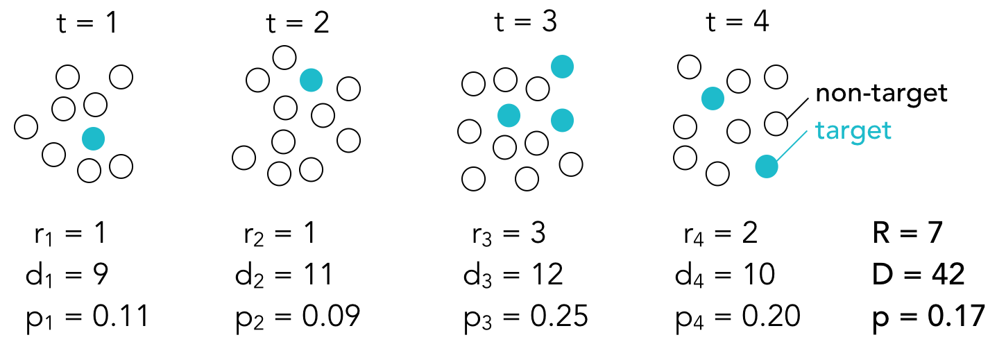
To find fads in the MRI literature, we can turn to burst detection. Burst detection finds periods of time in which a target is uncharacteristically popular, or, in other words, when it is "bursting." In our case, the target is one of the unique words in the dataset and we are looking for periods in which the word appears in a greater proportion of article titles than usual. The two-state model that I used assumes that a target can be in one of two states: a baseline state, in which the target occurs at some baseline or default rate, and a bursty state, in which the target occurs at an elevated rate. For every time point (in this case, for every month), the algorithm compares the frequency of the target at that time point to the frequency of the target over the full time period (the baseline rate) and tries to guess whether the target is in a baseline state or a bursty state. The algorithm returns its best guess of which state the target was in at each time point during the time period. In the example above, we would not expect carcinoma to enter a bursty state because the proportions don't get much greater than the baseline proportion (gray dotted line). However, we would expect connectivity to enter a burst state some time around 2014 because the proportions begin to far exceed the baseline proportion (blue dotted line).
There are a few parameters you can tweak in burst detection. The first is the "distance" between the baseline state and burst state. I used s=2 which means that a word has to occur with a frequency that is more than double its baseline frequency to be considered bursting. The second is the difficulty associated with moving up into a bursty state. I used gamma=0.5, which makes it relatively easy to enter a bursting state. Finally, I smoothed the time courses with a 5-month rolling window to reduce noise and facilitate the detection of the bursts. I applied the same burst detection model to all 6,310 unique words in the dataset to determine which terms, if any, were associated with bursts of activity and when those bursts occurred.
The vast majority of terms were not associated with any bursts, but a handful of terms did exhibit bursting activity. Below is a timeline of the top 100 bursts. Each bar represents one burst, with previous bursts in gray and current bursts (those that are still in a burst state as of November 2017) in blue. Since the time courses were smoothed, the start points and end points of the bursts are not precise (notice how the current bursts end in mid 2017).

This analysis reveals a beautiful progression in the MRI literature. Imaging-related terms trend early on, with tomography, computed, resonance, mr, magnetic, nmr, nuclear, imaging, and ct bursting in the late 1980s and early 1990s. Medical terms begin to appear in the mid-1990s, including tumors, findings, evaluation, and angiography. The early 2000s are punctuated by advances in MRI technology, as demonstrated by bursts in the terms fast, three-dimensional, gamma, knife, event-related, and tensor. Bursts after 2010 capture the cognitive revolution ushered in by fMRI, with bursts in the terms cognitive, social, connectivity, resting, state, altered, network, networks, resting-state, default, and mode.
To get an idea of how well the algorithm identified bursting periods, I plotted the proportions of the bursting words throughout the time period. Since there's great variability in the baseline proportions of the words, I normalized the monthly proportions by dividing them by each word's baseline proportion. Values of 1 indicate that the proportion is equal to the baseline proportion, values less that 1 (light blue) indicate that the proportion is less than the baseline, and values greater than 1 (dark blue) indicate that the proportion is greater than the baseline. The boundaries of the bursts are outline in black.

One thing that's apparent is that the burst detection algorithm does a poor job of detecting the beginning of the bursts. Take for example the terms fast, event-related, nephrogenic, state, pet/mr, and biomarker. I can think of a few explanations for this. First, it's possible that the algorithm identified multiple bursts, but the earlier bursts were not strong enough to enter the top 100 bursts. However, after looking at all of the bursts associated with the terms listed above, it doesn't look like any additional early bursts were detected. The second, more likely explanation, is that burst detection is simply ill-suited to detect early upticks in a topic. For example, if you look back to the time course of connectivity, it looks like the term begins to gain popularity around 2005 or so. However, up until 2011, the frequency of connectivity is less than the baseline frequency so the burst detection algorithm assumes it is in the baseline state. So instead of thinking of burst detection as a method that identifies when bubbles are forming, we should think of it as finding when bubbles burst or boil over (which is maybe when a fad starts anyway?)
CURRENT TRENDS
Since burst detection does a poor job of catching topics that are just beginning to become popular, I was curious about what topics are currently trending. To find the top trending words, I found the slope of the line of best fit of each word's proportions over the last two years. Words that appeared at the same rate throughout the time period should have slopes around zero, words that became less prevalent should have negative slopes, and words that became more prevalent should have positive slopes. After removing words with baseline proportions less than 0.005, I selected the top 15 words with the steepest upward slopes. The proportions of these words since 2015 is plotted below. (The trajectories are heavily smoothed to aid visualization, but they were not smoothed when computing the slopes.)

I think the lesson here is that if you want your research to be on the cutting edge, you need to write a paper titled "Accuracy and prognostic outcomes of simultaneous multi-parametric measurements for systematically predicting adolescents' resting-state networks and prostate cord fat." .... At least, I think that's the takeaway.
Finally, here are the top 15 words that have been rising in popularity over a longer 15 year period:

Connectivity is the obvious break out star, appearing in less than 0.5% of articles in 2002 and nearly 4% of articles in 2017.
I could probably make another half dozen graphs, but I'll stop myself here. Let me know what you thought about this analysis or if you have ideas about additional things to look at. Next I'm going to work on applying the same analysis to identifying trends in the New York Times news article archive.